DenseBoW


DenseBoW is a text classifier in fact it is a subclass of BoW being the difference the process to represent the text in a vector space. This process is described in “EvoMSA: A Multilingual Evolutionary Approach for Sentiment Analysis, Mario Graff, Sabino Miranda-Jimenez, Eric Sadit Tellez, Daniela Moctezuma. Computational Intelligence Magazine, vol 15 no. 1, pp. 76-88, Feb. 2020.” Particularly, in the section where the Emoji Space is described.
Dense BoW Representation
The idea is to represent a text in a vector space where the components have a more complex meaning than the BoW model. In BoW, each component’s meaning corresponds to the associated token, and the IDF value gives its importance.
The complex behavior comes from associating each component to the decision value of a text classifier (e.g., BoW) trained on a labeled dataset which is different from the task at hand, albeit nothing forbids to be related to it. The datasets from which these decision functions come can be built using a self-supervised approach or annotating texts.
Without loss of generality, it is assumed that there are \(M\) labeled datasets each one contains a binary text classification problem; noting that if a dataset has \(K\) labels, then this dataset can be represented as \(K\) binary classification problems following the one versus the rest approach, i.e., it is transformed to \(K\) datasets.
For each of these \(M\) binary text classification problems a BoW classifier is built using the default parameters (a pre-trained bag-of-words representation and a linear SVM as the classifier). Consequently, there are \(M\) binary text classifiers, i.e., \((c_1, c_2, \ldots, c_M)\). Additionally, the decision function of \(c_i\) is a value where the sign indicates the class. The text representation is the vector obtained by concatenating the decision functions of the \(M\) classifiers and then normalizing the vector to have length 1.
A text \(x\) is first represented with vector \(\mathbf{x^{'}} \in \mathbb R^M\) where the value \(\mathbf{x^{'}}_i\) corresponds to the decision function of \(c_i\). Given that the classifier \(c_i\) is a linear SVM, the decision function corresponds to the dot product between the input vector and the weight vector \(\mathbf w_i\) plus the bias \(\mathbf w_{i_0}\), where the weight vector and the bias are the parameters of the classifier. That is, the value \(\mathbf{x^{'}}_i\) corresponds to
where \(\mathbf{v_t}\) is the vector associated to the token \(t\) of the text \(x\). In matrix notation, vector \(\mathbf{x'}\) is
where matrix \(\mathbf W \in \mathbb R^{M \times d}\) contains the weights, and \(\mathbf{w_0} \in \mathbb R^M\) is the bias. Another way to see the previous formulation is by defining a vector \(\mathbf{u_t} = \frac{1}{\lVert \sum_k \mathbf{v_k} \rVert} \mathbf W \mathbf{v_t}\). Consequently, vector \(\mathbf{x'}\) is defined as
vectors \(\mathbf{u} \in \mathbb R^M\) correspond to the tokens; this is the reason we refer to this model as a dense BoW. Finally, the vector representing the text \(x\) is the normalized \(\mathbf{x^{'}}\), i.e.,
Parameters
The dense representations start by defining the labeled datasets used to create them. These datasets are organized in three groups. The first one is composed of human-annotated datasets; we refer to them as dataset. The second groups contain a set of self-supervised dataset where the objective is to predict the presence of an emoji as expected; these models are referred as emoji. The final group is also a set of self-supervised datasets where the task is to predict the presence of a particular word, namely keyword.
Following an equivalent approach used in the development of the pre-trained BoW, different dense representations were created; these correspond to varying the size of the vocabulary and the two procedures used to select the tokens.
Below is a table displaying the number of components for each dense representation group. It is worth noting that the dataset group is solely accessible for Arabic, English, Spanish, and Chinese. Additionally, the table indicates the number of tweets utilized in producing the self-supervised datasets, with a maximum of 100 million.
Language |
H.A. Datasets |
Emojis |
Keywords |
Number of Tweets |
|---|---|---|---|---|
Arabic (ar) |
30 |
465 |
2048 |
100.0 |
Catalan (ca) |
na |
136 |
2022 |
5.6 |
German (de) |
na |
199 |
2048 |
13.6 |
English (en) |
181 |
594 |
2048 |
100.0 |
Spanish (es) |
57 |
567 |
2048 |
100.0 |
French (fr) |
na |
549 |
2048 |
81.1 |
Hindi (hi) |
na |
176 |
2048 |
9.5 |
Indonesian (in) |
na |
366 |
2048 |
40.4 |
Italian (it) |
na |
260 |
2048 |
24.5 |
Japanese (ja) |
na |
450 |
1989 |
41.6 |
Korean (ko) |
na |
99 |
526 |
5.0 |
Dutch (nl) |
na |
157 |
2040 |
10.0 |
Polish (pl) |
na |
166 |
2040 |
10.8 |
Portuguese (pt) |
na |
471 |
2048 |
100.0 |
Russian (ru) |
na |
383 |
2048 |
100.0 |
Tagalog (tl) |
na |
242 |
2048 |
19.5 |
Turkish (tr) |
na |
380 |
2048 |
59.3 |
Chinese (zh) |
18 |
152 |
1953 |
5.6 |
The name of each component can be obtained from the attribute DenseBoW.names; for example, the following instructions retrieve the human-annotated datasets in Spanish.
>>> from EvoMSA import DenseBoW
>>> DenseBoW(lang='es', dataset=True,
             emoji=False, keyword=False).names
['HA(negative)', 'HA(neutral)', 'HA(positive)',
 'INEGI(1)', 'INEGI(2)', 'INEGI(3)', 'INEGI(4)',
 'meoffendes2021_task1(NO)', 'meoffendes2021_task1(NOM)',
 'meoffendes2021_task1(OFG)', 'meoffendes2021_task1(OFP)',
 'haha2018', 'tass2018_s1_l2', 'mexa3t2018_aggress',
 'tass2016(N)', 'tass2016(NEU)', 'tass2016(NONE)', 'tass2016(P)',
 'misogyny_centrogeo', 'meoffendes2021_task3',
 'detests2022_task1',
 'MeTwo(DOUBTFUL)', 'MeTwo(NON_SEXIST)', 'MeTwo(SEXIST)',
 'exist2021_task1', 'davincis2022_1', 'misoginia',
 'tass2018_s1_l1', 'delitos_ingeotec',
 'semeval2018_valence(-3)', 'semeval2018_valence(-2)',
 'semeval2018_valence(-1)', 'semeval2018_valence(0)',
 'semeval2018_valence(1)', 'semeval2018_valence(2)',
 'semeval2018_valence(3)', 'semeval2018_fear(0)',
 'semeval2018_fear(1)', 'semeval2018_fear(2)', 'semeval2018_fear(3)',
 'semeval2018_anger(0)', 'semeval2018_anger(1)', 'semeval2018_anger(2)',
 'semeval2018_anger(3)', 'semeval2018_sadness(0)', 'semeval2018_sadness(1)',
 'semeval2018_sadness(2)', 'semeval2018_sadness(3)', 'semeval2018_joy(0)',
 'semeval2018_joy(1)', 'semeval2018_joy(2)', 'semeval2018_joy(3)',
 'tass2017(N)', 'tass2017(NEU)', 'tass2017(NONE)', 'tass2017(P)',
 'tass2018_s2']
The notation includes the label between parentheses in case the dataset contains multiple classes. For binary classification, it only includes the dataset name, and the predicted label is the positive class.
Example
To illustrate the usage of these representations, the text I love this song is represented on the emoji space. The representation developed are pre-trained models; therefore, the vocabulary and language are fixed. The vocabulary size (\(2^d\)) is specified with the exponent \(d\) in the parameter voc_size_exponent; the default is \(17\). The language is defined in the parameter lang (default ‘es’). The examples presented use as defaults the following.
>>> SIZE = 15
>>> LANG = 'en'
The first step is to initialize the model which can be done with the following instructions.
>>> from EvoMSA import DenseBoW
>>> emoji = DenseBoW(lang=LANG,
                     voc_size_exponent=SIZE,
                     emoji=True,
                     keyword=False,
                     dataset=False)
The method DenseBoW.transform receives a list of text to be represented on this vector space, the following code stores the output matrix in the variable X.
>>> X = emoji.transform(['I love this song'])
Equivalent, the attribute DenseBoW.names contains the description of each component, for example the following code shows the value for the component with index 9 and its description.
>>> X[:, 59], emoji.names[59]
(array([0.08912432]), '🎶')
The value \(0.09`\) indicates that the emoji would be present in the sentence I love this song.
Text Classifier
As mentioned previously, DenseBoW is a subclass of BoW; consequently, once the text is in a vector space, the next step to create a text classifier is to train an estimator. In this case, it is a Linear Support Vector Machine.
To illustrate this process, we used a labeled dataset found in the EvoMSA; this set can be obtained with the following instructions.
>>> from microtc.utils import tweet_iterator
>>> from EvoMSA.tests.test_base import TWEETS
>>> import numpy as np
>>> D = list(tweet_iterator(TWEETS))
The dataset stored in D is a toy sentiment analysis dataset, in Spanish, with four labels, positive, negative, neutral, and none. It is a list of dictionaries where the dictionary has two keys text and klass; the former has the text and the latter the label.
Although one can directly provide the list of dictionaries to DenseBoW, it is decided to follow the conventions of sklearn. The following instructions transform D into the dependent variables and their response.
>>> X = [x['text'] for x in D]
>>> y = np.r_[[x['klass'] for x in D]]
The text classifier is trained with the following instruction.
>>> LANG = 'es'
>>> dense = DenseBoW(lang=LANG,
                     voc_size_exponent=SIZE,
                     emoji=True,
                     keyword=True,
                     dataset=False).fit(X, y)
where the language (lang) is set to Spanish (es), and fit receives the labeled dataset.
Note
It is equivalente to use the following code.
>>> dense = DenseBoW(lang=LANG,
                     voc_size_exponent=SIZE,
                     emoji=True,
                     keyword=True,
                     dataset=False).fit(D)
The method DenseBoW.predict is used to predict the label of a list of texts. For example, the label of the text buenos días (good morning) is computed as:
>>> dense.predict(['buenos días'])
array(['P'], dtype='<U4')
where the label ‘P’ corresponds to the positive class.
There are scenarios where it is more important to estimate the value(s) used to classify a particular instance; in the case of SVM, this is known as the decision function, and in the case of a Naive Bayes classifier, this is the probability of each class. This information can be found in DenseBoW.decision_function as can be seen in the following code.
>>> dense.decision_function(['buenos días'])
array([[-2.2368439 , -1.21958811, -0.4779458 ,  1.37261126]])
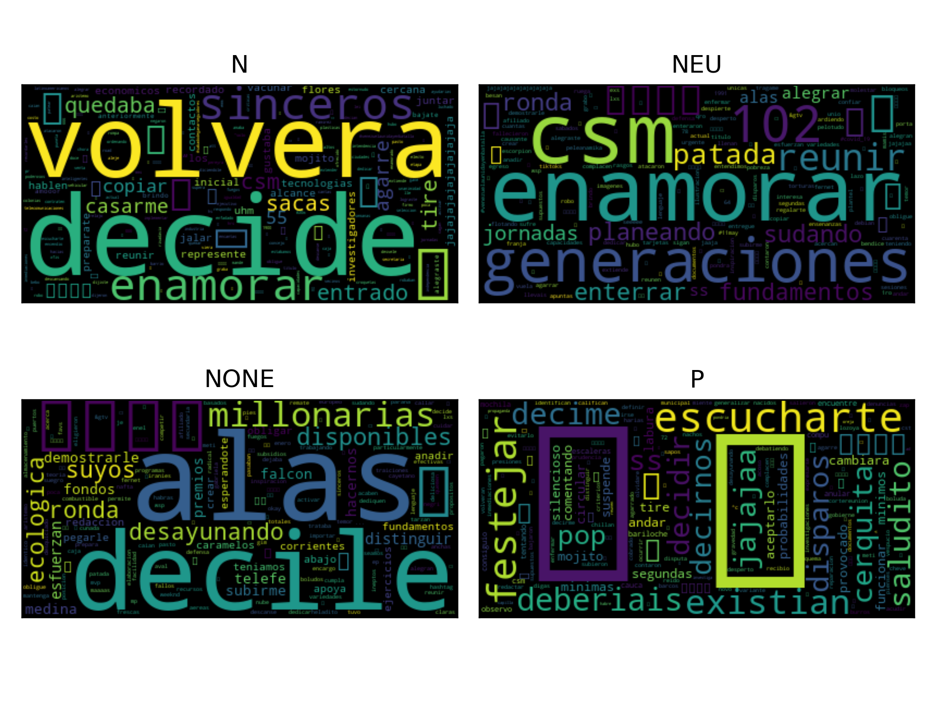
The text classifier used is a linear model where the value of the coefficients indicates the discriminant power of the feature in the text given; therefore, it is possible to create a word cloud to provide insight into the classification process. The dataset has four labels, so the classifier follows a strategy of one vs. the rest. Consequently, there are four binary classifiers, and the following figure presents the word cloud for the positive case in each classifier. The title of the figure indicates the label of the positive case for the word cloud. The procedure is equivalent to the one presented in Text Classifier, and the same example is used to facilitate a comparison.
>>> from wordcloud import WordCloud
>>> from matplotlib import pylab as plt
>>> txt = 'Es un placer estar aquí.'
>>> X = dense.transform([txt])
>>> clouds = []
>>> for ws in dense.estimator_instance.coef_:
>>>     positive = {name: w * repr
                    for name, repr, w in zip(dense.names,
                                              X[0], ws) if w * repr > 0}
>>>     _ = WordCloud().generate_from_frequencies(positive)
>>>     clouds.append(_)
>>> fig = plt.figure(dpi=300, tight_layout=True)
>>> axs = fig.subplots(2, 2).flatten()
>>> labels = np.unique(y)
>>> for cloud, ax, title in zip(clouds, axs, labels):
>>>     ax.imshow(cloud, interpolation='bilinear')
>>>     ax.grid(False)
>>>     ax.tick_params(left=False, right=False, labelleft=False,
                       labelbottom=False, bottom=False)
>>>     ax.set_title(title)