EvoMSA 2.0


EvoMSA is a stack generalization algorithm specialized in text classification problems. Text classification is a Natural Language Processing task focused on identifying a text’s category. A standard approach to tackle text classification problems is to pose it as a supervised learning problem. In supervised learning, everything starts with a dataset composed of pairs of inputs and outputs; in this case, the inputs are texts, and the outputs correspond to the associated labels or categories. The aim is that the developed algorithm can automatically assign a label to any given text independently, whether it was in the original dataset. The feasible categories are only those found on the original dataset. In some circumstances, the method can also inform the confidence it has in its prediction so the user can decide whether to use or discard it.
The key idea of EvoMSA is to combine different text classifiers using a stack generalization approach. A text classifier \(c\), can be seen as a composition of two functions, i.e., \(c \equiv g \circ m\); where \(m\) transforms the text into a vector space, i.e., \(m: \text{text} \rightarrow \mathbb R^d\) and \(g\) is the classifier (\(g: \mathbb R^d \rightarrow \mathbb N\)) or regressor (\(g: \mathbb R^d \rightarrow \mathbb R\)).
EvoMSA focused on developing diverse text representations (\(m\)), fixing the classifier \(g\) as a linear Support Vector Machine. The text representations (functions \(m\)) found in EvoMSA can be grouped into two. On the one hand, there is a traditional Bag of Words (BoW) representation; on the other, there is a dense representation, namely dense BoW.
EvoMSA 2.0 supports more languages than the previous version, currently it supports Arabic (ar), Catalan (ca), German (de), English (en), Spanish (es), French (fr), Hindi (hi), Indonesian (in), Italian (it), Japanese (ja), Korean (ko), Dutch (nl), Polish (pl), Portuguese (pt), Russian (ru), Tagalog (tl), Turkish (tr), and Chinese (zh).
EvoMSA 2.0 simplifies the previous version (EvoMSA), and now it has only three main classes.
BoW and DenseBoW are text classifiers; BoW is the parent of DenseBoW. The stack generalization technique is implemented in StackGeneralization.
EvoMSA 2.0 has been tested in many text classifier competitions without modifications. The aim is to offer a better understanding of how these algorithms perform in a new situation and what would be the difference in performance with an algorithm tailored to the new problem. In the following link, we will describe the specifics of each configuration.
Quickstart Guide
This section describes the usage of EvoMSA using a dummy text classification problem; mainly, it is a sentiment analysis dataset, in Spanish, with four labels: positive (P), negative (N), neutral (NEU), and none (NONE). The problem can be found in EvoMSA’s tests.
The guide includes the creation of three text classifiers, one using a BoW model, the other using a dense BoW, and the last classifier combines the previous two models using a stacking mechanism.
The first step is to install EvoMSA, which is described below.
Installing EvoMSA
The first step is to install the library, which can be done using the conda package manager with the following instruction.
conda install -c conda-forge EvoMSA
A more general approach to installing EvoMSA is through the use of the command pip, as illustrated in the following instruction.
pip install EvoMSA
Libraries and Text Classification Problem
Once EvoMSA is installed, one must load a few libraries. The first line loads EvoMSA core classes. Line 2 contains the pathname where the text classification problem is. Line 3 is a method to read a file containing a JSON per line. The rest of the lines are libraries used in the examples.
>>> from EvoMSA import BoW, DenseBoW, StackGeneralization
>>> from EvoMSA.tests.test_base import TWEETS
>>> from microtc.utils import tweet_iterator
>>> from IngeoML import SelectFromModelCV
>>> from CompStats import CI, StatisticSamples
>>> from CompStats import performance, difference, plot_difference
>>> from sklearn.model_selection import StratifiedKFold
>>> from sklearn.base import clone
>>> from sklearn import metrics
>>> import numpy as np
>>> import pandas as pd
>>> import seaborn as sns
>>> np.set_printoptions(precision=4)
>>> sns.set_style('whitegrid')
The text classification problem can be read using the following instruction. It is stored in a variable D which is a list of dictionaries. The second line shows the content of the first element in D.
>>> D = list(tweet_iterator(TWEETS))
>>> D[0]
{'text': '| R #OnPoint | #Summer16 ...... 🚣🏽🌴🌴🌴 @ Ocho Rios, Jamacia https://t.co/8xkfjhk52L',
 'klass': 'NONE',
 'q_voc_ratio': 0.4585635359116022}
The field text is self-described, and the field klass contains the label associated with that text. Although one can directly provide the list of dictionaries to BoW and DenseBoW, it is decided to follow the conventions of sklearn. The following instructions transform D into the dependent variables and their response.
>>> X = [x['text'] for x in D]
>>> y = np.r_[[x['klass'] for x in D]]
The text classifiers developed in the example are pre-trained models; therefore, the vocabulary and language are fixed. The vocabulary size (\(2^d\)) is specified with the exponent \(d\) in the parameter voc_size_exponent; the default is \(17\). The language is defined in the parameter lang (default ‘es’). The examples presented use as defaults the following.
>>> SIZE = 15
>>> LANG = 'es'
BoW Classifier
The first text classifier presented is the pre-trained BoW. The following line initializes the classifier, the first part initializes the class, and the second corresponds to the estimate of the parameters of the linear SVM.
>>> bow = BoW(lang=LANG,
              voc_size_exponent=SIZE).fit(X, y)
Note
It is equivalent to use the following instruction
>>> bow = BoW(lang=LANG,
              voc_size_exponent=SIZE).fit(D)
After training the text classifier, it can make predictions. For instance, the first line predicts the training set, while the second line predicts the phrase good morning in Spanish, buenos días.
>>> hy = bow.predict(D)
>>> bow.predict(['buenos días'])
array(['P'], dtype='<U4')
It can be observed that the predicted class for buenos días is positive (P).
In order to measure the text classifier performance in this dataset, a stratified k-fold cross-validation can be used. The first step is to create a clean instance of BoW with the following instruction.
>>> bow = BoW(lang=LANG,
              voc_size_exponent=SIZE)
The next step is to implement the k-fold strategy with the following instructions.
>>> hy_bow = np.empty_like(y)
>>> skf = StratifiedKFold(shuffle=True, random_state=0)
>>> for tr, vs in skf.split(X, y):
>>>     m = clone(bow).fit([X[x] for x in tr], y[tr])
>>>     hy_bow[vs] = m.predict([X[x] for x in vs])
Finally, the performance (\(f_1\) score) for the different labels can be computed as follows.
>>> metrics.f1_score(y, hy_bow, average=None)
array([0.5595, 0.    , 0.3741, 0.7474])
In order to complement the point performance obtained in the previous instruction, the confidence interval can be computed with the following instructions.
>>> f1 = lambda y, hy: metrics.f1_score(y, hy,
                                        average=None)
>>> statistic = StatisticSamples(statistic=f1)
>>> samples = statistic(y, hy_bow)
>>> CI(samples)
(array([0.4989, 0.    , 0.3112, 0.7173]),
 array([0.6081, 0.    , 0.4486, 0.7707]))
DenseBoW Classifier
Next, the second method is trained using the dataset following the same steps. The subsequent instruction shows the code to train the text classifier.
>>> dense = DenseBoW(lang=LANG,
                     voc_size_exponent=SIZE,
                     emoji=True,
                     keyword=True,
                     dataset=False).fit(X, y)
Note
It is equivalente to use the following code.
>>> dense = DenseBoW(lang=LANG,
                     voc_size_exponent=SIZE,
                     emoji=True,
                     keyword=True,
                     dataset=False).fit(D)
The code to predict is equivalent; therefore, the prediction for the phrase good morning is only shown.
>>> dense.predict(['buenos días'])
array(['P'], dtype='<U4')
In order to measure the text classifier performance in this dataset, a stratified k-fold cross-validation can be used. The first step is to create a clean instance of DenseBoW with the following instruction.
>>> dense = DenseBoW(lang=LANG,
                     emoji=True,
                     keyword=True,
                     dataset=False,
                     voc_size_exponent=SIZE)
The next step is to implement the k-fold strategy with the following instructions.
>>> hy_dense = np.empty_like(y)
>>> skf = StratifiedKFold(shuffle=True, random_state=0)
>>> for tr, vs in skf.split(X, y):
>>>     m = clone(dense).fit([X[x] for x in tr], y[tr])
>>>     hy_dense[vs] = m.predict([X[x] for x in vs])
Finally, the performance (\(f_1\) score) for the different labels can be computed as follows.
>>> metrics.f1_score(y, hy_dense, average=None)
array([0.6208, 0.    , 0.4828, 0.7679])
In order to complement the point performance obtained in the previous instruction, the confidence interval can be computed with the following instructions.
>>> f1 = lambda y, hy: metrics.f1_score(y, hy, average=None)
>>> statistic = StatisticSamples(statistic=f1)
>>> samples = statistic(y, hy_dense)
>>> CI(samples)
(array([0.5683, 0.    , 0.4131, 0.7377]),
 array([0.6679, 0.    , 0.5463, 0.7927]))
It is also possible to select the most discriminant features for the problem being solved. The method SelectFromModelCV is used in the following example. The first step is to create a clean instance of DenseBoW. The following lines define the parameters for the class SelectFromModelCV. Finally, the feature selection is performed on the method select.
>>> dense = DenseBoW(lang=LANG,
                     emoji=True,
                     keyword=True,
                     dataset=False,
                     voc_size_exponent=SIZE)
>>> macro_f1 = lambda y, hy: metrics.f1_score(y, hy,
                                              average='macro')
>>> kwargs = dense.estimator_kwargs
>>> estimator = dense.estimator_class(**kwargs)
>>> kwargs = dict(estimator=estimator,
                  scoring=macro_f1)
>>> dense.select(D=X, y=y,
                 feature_selection=SelectFromModelCV,
                 feature_selection_kwargs=kwargs)
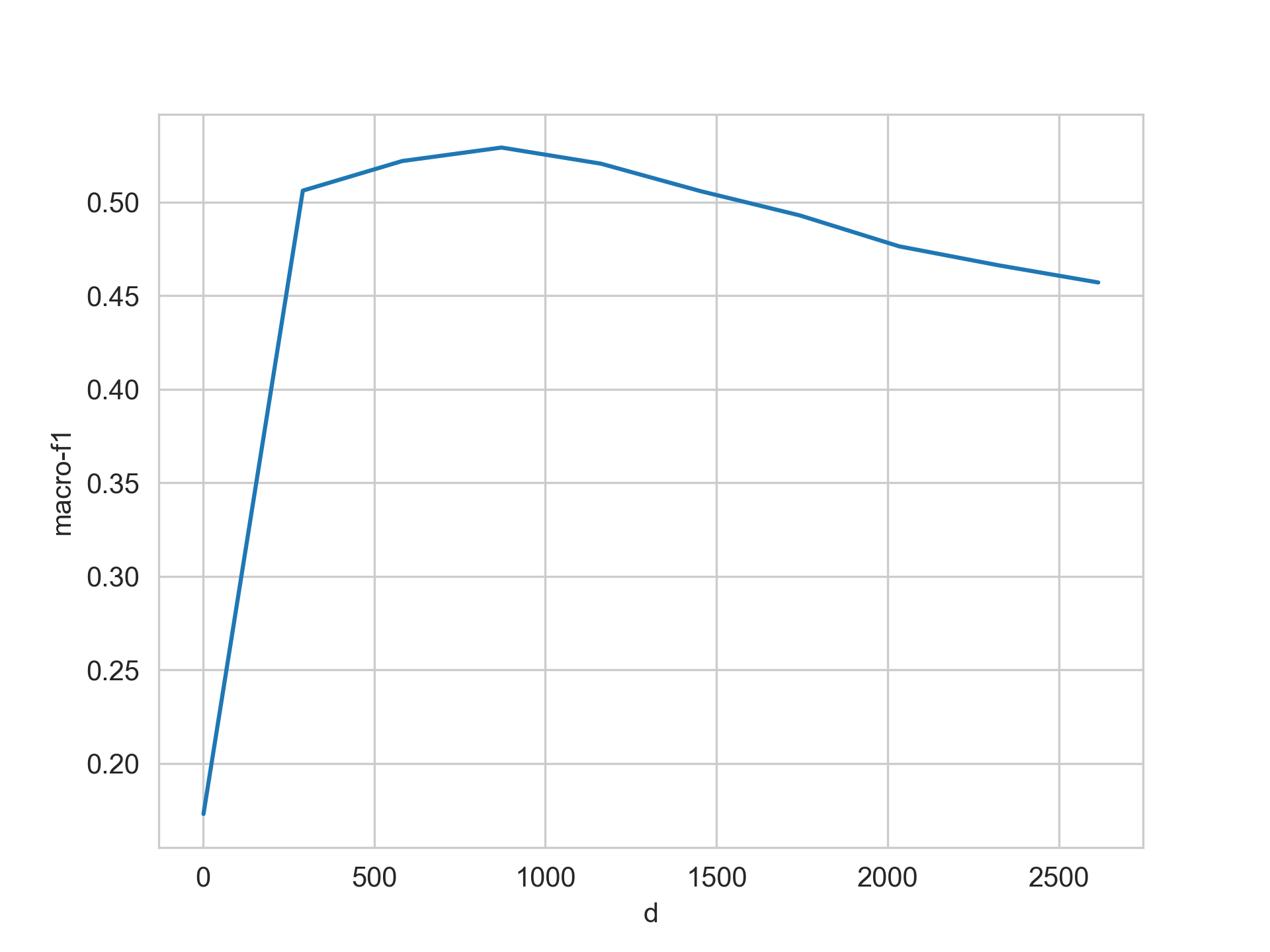
The performance for the selected features can be retrieved with the following instructions. The figure shows the performance when the number of features is varied.
>>> select = dense.feature_selection
>>> perf = select.cv_results_
>>> _ = [{'d': k, 'macro-f1': v} for k, v in perf.items()]
>>> df = pd.DataFrame(_)
>>> ax = sns.lineplot(df, x='d', y='macro-f1')
The performance of the text classifier enhanced with the feature selection algorithm can be computed with the following instructions.
>>> dense = DenseBoW(lang=LANG,
                     emoji=True,
                     keyword=True,
                     dataset=False,
                     voc_size_exponent=SIZE)
>>> hy = np.empty_like(y)
>>> skf = StratifiedKFold(shuffle=True, random_state=0)
>>> for tr, vs in skf.split(X, y):
>>>     m = clone(dense).select(D=[X[x] for x in tr], y=y[tr],
                                feature_selection=SelectFromModelCV,
                                feature_selection_kwargs=kwargs)
>>>     m.fit([X[x] for x in tr], y[tr])
>>>     hy[vs] = m.predict([X[x] for x in vs])
>>> metrics.f1_score(y, hy, average=None)
array([0.6324, 0.    , 0.521 , 0.766 ])
Stack Generalization
The final text classifier uses a stack generalization approach. The first step is to create the base text classifiers corresponding to the two previous text classifiers, BoW, and DenseBoW.
>>> bow = BoW(lang=LANG,
              voc_size_exponent=SIZE)
>>> dense = DenseBoW(lang=LANG,
                     emoji=True,
                     keyword=True,
                     dataset=False,
                     voc_size_exponent=SIZE)
It is worth noting that the base classifiers were not trained; as can be seen, the method fit was not called. These base classifiers will be trained inside the stack generalization algorithm.
The second step is to initialize and train the stack generalization class, shown in the following instruction.
>>> stack = StackGeneralization([bow, dense]).fit(X, y)
Note
It is equivalent to use the following instruction.
>>> stack = StackGeneralization([bow, dense]).fit(D)
One does not need to specify the language to stack generalization because the base text classifiers give the language.
The code to predict is kept constant in all the classes; therefore, the following code predicts the class for the phrase good morning.
>>> stack.predict(['buenos días'])
array(['P'], dtype='<U4')
In order to measure the text classifier performance in this dataset, a stratified k-fold cross-validation can be used. The first step is to create a clean instance of StackGeneralization with the following instruction.
>>> bow = BoW(lang=LANG,
              voc_size_exponent=SIZE)
>>> dense = DenseBoW(lang=LANG,
                     emoji=True,
                     keyword=True,
                     dataset=False,
                     voc_size_exponent=SIZE)
>>> stack = StackGeneralization([bow, dense])
The next step is to implement the k-fold strategy with the following instructions.
>>> hy_stack = np.empty_like(y)
>>> skf = StratifiedKFold(shuffle=True, random_state=0)
>>> for tr, vs in skf.split(X, y):
>>>     m = clone(stack).fit([X[x] for x in tr], y[tr])
>>>     hy_stack[vs] = m.predict([X[x] for x in vs])
Finally, the performance (\(f_1\) score) for the different labels can be computed as follows.
>>> metrics.f1_score(y, hy_stack, average=None)
array([0.6445, 0.08  , 0.5181, 0.7426])
In order to complement the point performance obtained in the previous instruction, the confidence interval can be computed with the following instructions.
>>> f1 = lambda y, hy: metrics.f1_score(y, hy, average=None)
>>> statistic = StatisticSamples(statistic=f1)
>>> samples = statistic(y, hy_stack)
>>> CI(samples)
(array([0.5973, 0.    , 0.4605, 0.7138]),
 array([0.6883, 0.24  , 0.5748, 0.7728]))
Comparison
It is important to note that the dataset is synthetic and must be used in any practical application; however, one can use it to compare the different text classifiers trained. The variables hy_bow, hy_dense, and hy_stack have the predictions of each text classifier, so the following line sets these predictions and the actual labels in a data frame.
>>> df = pd.DataFrame(dict(BoW=hy_bow,
                           Dense=hy_dense,
                           Stack=hy_stack,
                           y=y))
The next step is to define the performance score. The macro-f1 score is used in this case, as seen in the following line.
>>> macro_f1 = lambda y, hy: metrics.f1_score(y, hy, average='macro')
>>> perf = performance(df, score=macro_f1)
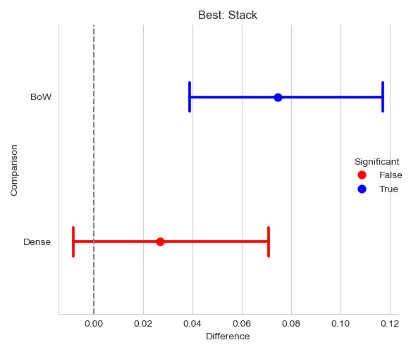
The final step is to estimate the difference in performance between the best system and the rest, as seen in the following lines. The figure shows the difference in performance between the best system StackGeneralization and the other text classifiers, namely BoW and DenseBoW. The DenseBoW classifier is in red to indicate that it is statistically equivalent to the StackGeneralization classifier.
>>> diff = difference(perf)
>>> plot_difference(diff)
Citing
If you find EvoMSA useful for any academic/scientific purpose, we would appreciate citations to the following reference:
@article{DBLP:journals/corr/abs-1812-02307,
author = {Mario Graff and Sabino Miranda{-}Jim{\'{e}}nez
               and Eric Sadit Tellez and Daniela Moctezuma},
title     = {EvoMSA: {A} Multilingual Evolutionary Approach for Sentiment Analysis},
journal   = {Computational Intelligence Magazine},
volume    = {15},
issue     = {1},
year      = {2020},
pages     = {76 -- 88},
url       = {https://ieeexplore.ieee.org/document/8956106},
month     = {Feb.}
}
API
EvoMSA first version
The documentation of EvoMSA first version can be found in the following sections.